Linear Programming Project: Product Mix and Diet Models With Graphs

A linear programming project begins with an everyday question: when several choices compete for limited resources, what is the best combination?

A workshop cannot make unlimited products because time, material, storage, and demand are limited. A meal plan cannot use unlimited quantities because cost, nutrition, and serving limits matter. Linear programming turns these practical restrictions into inequalities, draws the choices that remain possible, and then finds the best one.

That is why a strong project should do more than show a neat graph. It should tell a believable story from beginning to end:

1. define the decision clearly
2. translate the situation into variables and constraints
3. draw the common feasible region
4. calculate its corner points exactly
5. test the objective function
6. interpret the result in ordinary language
7. discuss assumptions and limitations honestly

This guide develops a complete product-mix project using a small desk-accessory workshop. It also shows how to adapt the same structure into a diet model if you prefer a cost-minimisation topic.

What the Finished Project Should Contain

Use a simple order that an examiner can follow without searching for missing steps.

Project section	What to include
Title page	Topic, name, class, school, session, and subject
Acknowledgement	A short, genuine note of thanks
Certificate	Only in the format required by your school
Index	Headings with page numbers
Introduction	Meaning, purpose, and uses of linear programming
Objectives	What your project will formulate, solve, and interpret
Key terms	Decision variables, constraints, objective, feasible region, optimum
Data and assumptions	The fictional or observed situation being modelled
Mathematical formulation	Variables, inequalities, non-negativity, and objective function
Graphical solution	Boundary table, scale, shaded region, and labelled corners
Calculations	Exact intersections and objective-value table
Findings	Best mix, best value, used resources, and unused resources
Limitations	What the two-variable linear model leaves out
Conclusion	One short answer to the original project question
Bibliography	Sources actually used
Viva preparation	Questions you can answer in your own words

The current official Mathematics project guidance treats project work as 20 marks across two projects and assesses each project through overall format, content, findings, and viva voce. It also expects a linear programming project to cover terminology, formulation, the graphical method, feasible and infeasible regions, optimum solutions, applications, advantages, and limitations. That makes your explanation and interpretation just as important as the final corner-point table.

Ready Project Title

You may use:

Using Linear Programming to Find the Profit-Maximising Product Mix for a Small Desk-Accessory Workshop

This title states the method, the decision, the setting, and the objective. It is more useful than a vague title such as “Linear Programming Project.”

If you choose the diet alternative later in this guide, use:

Using Linear Programming to Find a Minimum-Cost Cafeteria Meal Combination

Introduction You Can Adapt

Linear programming is a mathematical method for choosing the best value of a linear objective function while satisfying a set of linear constraints. The quantities that must be chosen are called decision variables. Restrictions on resources or requirements become inequalities. Every point satisfying all the inequalities is a feasible solution, and all such points together form the feasible region.

In a two-variable problem, the constraints can be represented on a graph. The maximum or minimum value is then checked at the corner points of the feasible region. This project applies that method to a workshop that makes two products using limited cutting time, finishing time, and daily packing capacity.

Linear programming is used in production planning, transport, scheduling, blending, agriculture, and cost control. Its value lies in making the trade-off between competing uses of limited resources visible and measurable.

Objectives of the Project

1. To understand the practical meaning of decision variables, constraints, a feasible region, and an objective function.
2. To formulate a product-mix situation as a linear programming problem in two variables.
3. To draw the constraints and identify the common feasible region.
4. To calculate all feasible corner points exactly.
5. To find the product mix that gives maximum daily profit.
6. To identify which resources are fully used and which have spare capacity.
7. To recognise the assumptions and limitations of the model.

The Product-Mix Story

Suppose a small workshop makes two wooden desk accessories:

• desk trays, which need more cutting work
• pen stands, which need more finishing work

The workshop records its daily capacities in simple resource units. These figures are designed for a school model, so they keep the arithmetic readable while still creating a meaningful feasible region.

Item	Desk tray	Pen stand	Daily capacity
Cutting units	2	1	100
Finishing units	1	2	80
Packing places	1	1	55
Profit per unit	Rs 80	Rs 70	Not applicable

Assume that every completed item can be sold, profit per unit remains constant, resources are used in the stated proportions, and fractional production is not intended in the final recommendation.

Step 1: Define the Decision Variables

Let:

x = number of desk trays made per day
y = number of pen stands made per day

Writing the units matters. If x meant rupees in one paragraph and number of trays in another, the entire model would lose meaning.

Since the workshop cannot make a negative quantity:

x >= 0 and y >= 0

These are the non-negativity restrictions.

Step 2: Form the Constraints

Cutting constraint

Each tray uses 2 cutting units and each pen stand uses 1. At most 100 units are available.

2x + y <= 100

Finishing constraint

Each tray uses 1 finishing unit and each pen stand uses 2. At most 80 units are available.

x + 2y <= 80

Packing constraint

Each product needs one packing place, and only 55 places are available per day.

x + y <= 55

All three use <= because they describe maximum available capacity. The workshop may leave a resource unused, but it cannot exceed the limit.

Step 3: Write the Objective Function

The workshop earns Rs 80 on each tray and Rs 70 on each pen stand. Therefore, daily profit is:

P = 80x + 70y

The objective is to maximise P subject to all the constraints.

The complete model is:

Maximise P = 80x + 70y

subject to
2x + y <= 100
x + 2y <= 80
x + y <= 55
x >= 0, y >= 0

Step 4: Prepare a Boundary Table

Replace each inequality with equality and find two points on each line.

Boundary line	Point 1	Point 2
2x + y = 100	(50, 0)	(25, 50)
x + 2y = 80	(0, 40)	(40, 20)
x + y = 55	(55, 0)	(0, 55)

Choose a scale that can show values from 0 to 60 on both axes. For example, 1 cm may represent 10 units. Label the horizontal axis x, the vertical axis y, and write the scale below the graph.

The origin (0, 0) satisfies all three capacity inequalities, so the allowed side of each line contains the origin. The required area is the common overlap in the first quadrant.

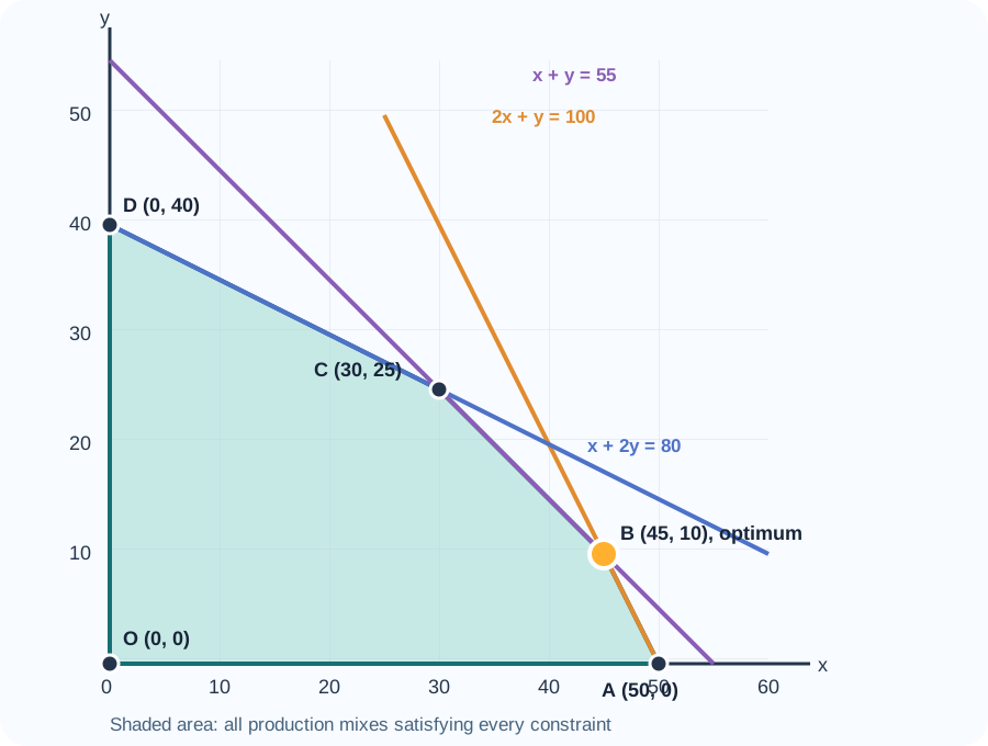
For a detailed refresher on test points, false intersections, bounded regions, and corner tables, read Linear Programming Graphs: Feasible Regions and Corner Points.

Step 5: Find Every Corner Point Exactly

Read the feasible boundary in order:

O(0, 0), A(50, 0), B, C, D(0, 40)

Point A lies on the x-axis. With y = 0, the three limits give x <= 50, x <= 80, and x <= 55. The smallest limit is 50, so A = (50, 0).

Point D lies on the y-axis. With x = 0, the limits give y <= 100, y <= 40, and y <= 55. The smallest limit is 40, so D = (0, 40).

Find B from the cutting and packing lines

2x + y = 100
x + y = 55

Subtract the second equation from the first:
x = 45

Then y = 55 - 45 = 10

B = (45, 10)

Check the finishing condition:

x + 2y = 45 + 20 = 65 <= 80

So B is feasible.

Find C from the finishing and packing lines

x + 2y = 80
x + y = 55

Subtract the second equation from the first:
y = 25

Then x = 55 - 25 = 30

C = (30, 25)

Check the cutting condition:

2x + y = 60 + 25 = 85 <= 100

So C is feasible.

Reject the intersection that lies outside

The cutting and finishing boundaries meet at (40, 20):

2x + y = 100
x + 2y = 80

Solving gives x = 40 and y = 20.

But x + y = 60, which exceeds the packing limit of 55. Therefore, (40, 20) is not a feasible corner and must not enter the profit table.

Step 6: Evaluate the Objective at the Feasible Corners

Corner	Calculation of P = 80x + 70y	Daily profit
O (0, 0)	80(0) + 70(0)	Rs 0
A (50, 0)	80(50) + 70(0)	Rs 4,000
B (45, 10)	80(45) + 70(10)	Rs 4,300
C (30, 25)	80(30) + 70(25)	Rs 4,150
D (0, 40)	80(0) + 70(40)	Rs 2,800

The greatest value is Rs 4,300 at B.

Therefore, the workshop should make 45 desk trays and 10 pen stands per day to earn a maximum daily profit of Rs 4,300 under the assumptions of the model.

OpenStax presents the same four-part logic for two-variable linear programming: create the objective, create the constraints, graph their common region, and evaluate the objective at the corner points. The important part of a project is to show how each algebraic step still means something in the original situation.

Step 7: Turn the Answer Into Findings

Do not end with only “maximum at B.” Translate the result back into the workshop.

At (45, 10):

Resource	Used	Available	Spare capacity
Cutting	2(45) + 10 = 100	100	0
Finishing	45 + 2(10) = 65	80	15
Packing	45 + 10 = 55	55	0

This supports four useful findings:

1. Cutting capacity and packing capacity are fully used at the optimum.
2. Finishing has 15 unused units, so it is not the immediate bottleneck.
3. Increasing finishing capacity alone would not improve the answer while the other limits remain unchanged.
4. The best mix contains both products. Producing only trays gives Rs 4,000, while producing only pen stands gives Rs 2,800.

A Small Sensitivity Check

A thoughtful project can ask whether a small change would alter the decision.

Keep tray profit at Rs 80 and call pen-stand profit q. At B, profit is:

80(45) + 10q = 3600 + 10q

At neighbouring corner A, profit is 80(50) = 4000. B is at least as good as A when:

3600 + 10q >= 4000
q >= 40

At neighbouring corner C, profit is 80(30) + 25q = 2400 + 25q. B is at least as good as C when:

3600 + 10q >= 2400 + 25q
q <= 80

So B remains optimal while pen-stand profit lies between Rs 40 and Rs 80 per unit. At an endpoint, two neighbouring corners may give the same maximum. This is not required for the basic graphical solution, but it shows that an optimum can remain stable over a range of profit estimates.

How to Convert This Into a Diet Project

The structure remains the same, but the signs often change.

Let:

x = number of servings of food A
y = number of servings of food B

Suppose a cafeteria wants to minimise cost while meeting stated minimum requirements. A general model may look like this:

Minimise C = ax + by

subject to
protein contribution >= minimum protein requirement
fibre contribution >= minimum fibre requirement
x + y <= practical serving limit
x >= 0, y >= 0

The first two constraints use >= because the nutrients must reach a minimum. The serving cap uses <= because it is a maximum. The feasible region may lie away from the origin, since (0, 0) cannot meet a positive minimum requirement.

MIT’s linear programming notes introduce the diet problem by choosing food quantities as variables, minimising their total cost, and requiring each nutrient total to meet a stated minimum. That is the mathematical idea your project may adapt.

However, your data should be handled carefully:

• use the same serving unit for both foods
• cite the label, official database, or other reliable source of nutrient figures
• state whether values are rounded
• avoid making medical claims
• do not call the result a complete or healthy diet merely because it satisfies two chosen constraints
• add realistic upper limits if unlimited servings would make the model silly

Product Mix or Diet Model: Which Should You Choose?

Consideration	Product-mix project	Diet project
Objective	Usually maximise profit or output	Usually minimise cost
Common signs	Resource limits often use <=	Minimum requirements often use >=
Data collection	Time, material, demand, and profit estimates	Serving cost and nutrient data
Main risk	Inventing unrealistic capacities or profit	Treating a simplified model as health advice
Interpretation	Best production combination and spare resources	Least-cost combination meeting selected conditions

Choose the model you can explain confidently. A modest project with clear assumptions is stronger than a complicated project whose data and units you do not understand.

Assumptions to State Clearly

The product-mix solution depends on these assumptions:

1. Profit per unit remains Rs 80 and Rs 70 throughout the relevant range.
2. Resource use per item remains constant.
3. All items produced can be sold.
4. Only the three stated capacities restrict production.
5. Production is completed within one day.
6. Product quality does not change as output changes.
7. The workshop can produce the recommended whole-number quantities.

These assumptions are not hidden weaknesses. They define the boundary within which your conclusion is valid.

Limitations of the Model

• Real profit may change with discounts, waste, overtime, or bulk purchases.
• Demand may be uncertain rather than fixed.
• Workers and machines may not operate at constant speed.
• A two-variable graph cannot directly handle many products.
• Some decisions require whole numbers, while an ordinary graphical model allows any real point.
• Important non-quantitative factors such as quality, fatigue, supplier reliability, and customer preference are omitted.
• The model describes one set of capacities and should be recalculated when the data changes.

Linear programming is powerful because it simplifies a decision, but the simplification must remain visible.

Common Project Mistakes

Writing inequalities without explaining them

Every coefficient should come from the table or story. Write one sentence for each constraint.

Shading each inequality but not the common overlap

The feasible region is the set of points satisfying all constraints together.

Using every line intersection as a corner

Substitute each candidate into every inequality. The point (40, 20) in this project fails the packing condition.

Reading corners only from a thick graph line

Use the graph to locate them, then solve simultaneous equations for exact coordinates.

Forgetting units

State that (45, 10) means 45 trays and 10 pen stands, and that Rs 4,300 is daily profit.

Claiming that unused capacity proves the answer is wrong

An optimum may leave some resources unused. The model requires the best feasible result, not full use of every resource.

Copying a project you cannot defend

Viva questions quickly reveal whether you understand the variables, signs, scale, and final interpretation. Adapt the setting and write in your own voice.

Viva Questions With Short Answers

What is the objective function in this project?

It is P = 80x + 70y, which represents the daily profit to be maximised.

Why are the constraints linear?

Each product uses a constant amount of each resource, so total use is a first-degree expression in x and y.

Why do we use non-negativity constraints?

Negative quantities of physical products have no meaning in this situation.

What is a feasible solution?

It is any pair (x, y) satisfying every capacity and non-negativity condition.

Why is (40, 20) rejected?

It satisfies the cutting and finishing equalities but needs 60 packing places, which exceeds the limit of 55.

Which constraints are binding at the optimum?

The cutting and packing constraints are binding because both are used fully at (45, 10).

Does spare finishing capacity mean finishing should be removed from the model?

No. It still limits other feasible combinations even though it is not fully used at the optimum.

Can the answer change if profits change?

Yes. The feasible region stays the same if capacities stay fixed, but a changed objective function may make another corner best.

Conclusion You Can Adapt

This project formulated a workshop’s production decision as a two-variable linear programming problem. The graphical method produced five feasible corner points. Evaluating the profit function at those points showed that 45 desk trays and 10 pen stands give the maximum daily profit of Rs 4,300 under the stated assumptions. At this combination, cutting and packing capacities are fully used, while 15 finishing units remain spare.

The model demonstrates how linear programming converts limited resources and competing choices into a clear decision. It also shows why the final answer should be read together with the assumptions, resource use, and limitations rather than as an isolated number.

Sources and Further Reading

• Official Mathematics syllabus and project guidance, for the project structure, assessment, and expected linear programming coverage.
• OpenStax, Linear Programming, for formulation, graphical solution, and corner-point evaluation.
• MIT OpenCourseWare, Linear Programming notes, for the diet formulation and broader applications.

Frequently Asked Questions

1. Can I use fictional data in a linear programming project?

Yes, if your teacher allows it and you label the data as illustrative. Do not claim that invented figures came from a real business or survey.

2. Should I choose a product-mix project or a diet project?

Choose the one whose data, units, and assumptions you can explain most confidently. Product mix is often easier to interpret, while a diet model gives useful practice with minimum requirements.

3. How many variables should a graphical project use?

Use two decision variables. More variables cannot be displayed directly on an ordinary two-dimensional graph.

4. Must the feasible region always contain the origin?

No. Capacity constraints with <= often include it, but minimum requirements with >= often exclude it.

5. Why do we evaluate the objective function at corner points?

For a linear objective over a polygonal feasible region, an optimum, when it exists, occurs at a corner or along an edge joining optimal corners.

6. What if two corner points give the same maximum value?

Then every feasible point on the line segment joining those corners also gives the same maximum value.

7. Can a feasible region be unbounded?

Yes. An unbounded region may still have an optimum for a particular objective, but it needs an additional check rather than an automatic conclusion.

8. What if the optimum has a fractional number of products?

Explain that physical products may require whole numbers. Test nearby feasible integer points, or state that integer programming would model the restriction more accurately.

9. Should graph coordinates be estimated or calculated?

Use the graph to identify likely corners, but calculate non-obvious intersections algebraically so your values are exact.

10. Do I need to include unused resources?

It is strongly recommended. Spare-capacity calculations turn a mathematical answer into a useful business finding.

11. Can I make the graph with software?

Follow your teacher’s instructions. Even if software is allowed, show the equations, scale, corner calculations, and interpretation yourself.

12. What is the most important viva preparation?

Be ready to explain what x and y mean, why each inequality has its sign, how each corner was found, why one intersection was rejected, and what the final answer means in the original situation.